

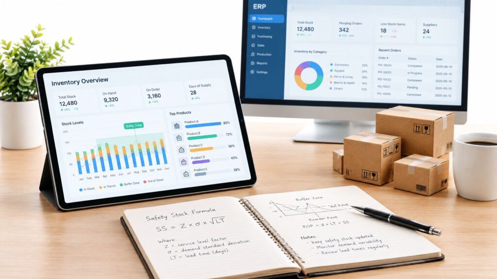
Your forecast looks reasonable. The supplier usually delivers when promised. Then demand jumps while a delivery slips, and the warehouse runs short before purchasing can respond. The safety stock formula helps you set a buffer for that gap, but the calculation only works when your planning system uses the right demand history, lead times, and item policy.
What Safety Stock Actually Protects You From
Safety stock is extra inventory held to absorb uncertainty during replenishment. It protects against the difference between what you expect to consume and what you need before replacement stock becomes available.
That’s different from cycle stock, which covers ordinary consumption between replenishments. If a planner expects an item to move steadily, the normal replenishment quantity supports that expected use. The safety buffer covers the variation around it.
A forecast can be useful without being exact. Likewise, a supplier can be dependable without delivering every order within an identical window. Treating all variation as a planning failure encourages teams to chase impossible precision instead of making a clear risk decision.
Practical rule: Set the buffer to protect a defined business commitment, not to hide every weakness in the supply chain.
The business commitment matters. A shortage of an easily substituted item creates a different problem from a missing component that stops production. Operations managers should involve purchasing, sales, and finance when deciding which consequences justify additional inventory.
For teams evaluating where to allocate protection across operations, Forge Reliability on reliability consulting offers a related resource for considering resource allocation. The practical question is which operational risks deserve scarce resources, including inventory.
A useful buffer balances holding cost against shortage consequences. It isn’t an emergency pile that nobody questions, and it isn’t a statistical result that automatically becomes policy. Someone must own the decision, document the reasoning, and revisit it when the operating conditions change.
How Safety Stock Fits Into Reorder Point Logic
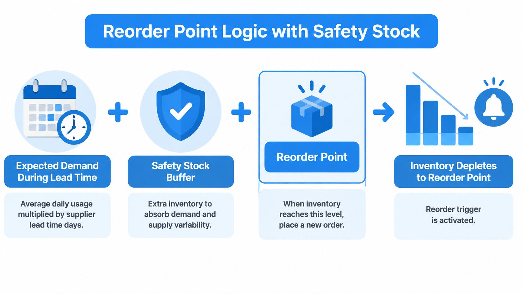
The reorder point answers when replenishment should begin. Safety stock answers how much protection to add for uncertainty. Keeping those decisions separate prevents a common configurationConfiguration sets up software using its existing options. In an ERP system, it adapts workflows, roles and other settings to the company's business processes. error.
For the fixed-lead-time model, ROPROP (reorder point) is the inventory level that signals when to replenish stock, based on expected demand during supplier lead time and the safety stock needed to reduce stockout risk. = μd × L + SS, where μd is average demand per period, L is replenishment lead time in matching periods, and SS is the uncertainty buffer. The distinction between expected demand and safety stock follows the statistical approach described in MIT’s safety-stock reference.
The expected-demand term supports consumption while the replacement order is being fulfilled. The buffer sits above that expected requirement. If you configure safety stock as though it were the entire lead-time requirement, you mix normal usage with protection and make the planning rule harder to validate.
Define the trigger before automating it
Document what your system compares with the reorder point. A simple on-hand trigger needs controls for open purchase orders and existing commitments. Otherwise, a planner may propose another order even though enough replenishment is already due.
Also define when stock counts as available. Goods awaiting inspection or put away may not yet support picking or production.
The order quantity remains a separate decision. Crossing the threshold should initiate the replenishment process, not dictate a purchase quantity without considering packaging, supplier minimums, and the item’s ordering policy. A mathematically correct buffer won’t rescue an unclear replenishment rule.
The Standard Formula With Fixed Lead Time
Use the standard calculation when demand varies but replenishment lead time is effectively fixed:
SS = Z × σd × √L
The formula uses the statistical approach cited above. Its inputs must describe the same item, location, and operating conditions.
- Z is the service factor. It represents the chosen cycle service target under the normal-distribution model.
- σd is demand standard deviation. It measures variation in demand per period, not average consumption.
- L is lead time. Express it in the same periods used to calculate demand variability.
Work through the demand buffer
In Amazon Business’s safety-stock example, average demand is 20 units per day, daily demand standard deviation is 5 units, lead time is 9 days, and the service target is 95%, using Z ≈ 1.65. The calculation is 1.65 × 5 × √9 = 1.65 × 5 × 3, giving approximately 25 units after rounding.
Average demand doesn’t enter this buffer calculation. It belongs in expected lead-time demand. The square-root term scales daily uncertainty across the replenishment window rather than multiplying it directly by elapsed time.
Don’t replace standard deviation with average sales just because the average is easier to extract from your system.
Know what the service target means
The example’s target is a cycle service level, not a fill-rate commitment. Most inventory-management tutorials define the service factor in terms of standard deviations above average lead-time demand. The target concerns avoiding a stockout during a replenishment cycle, rather than the share of individual units supplied without delay.
Before using this formula, inspect the demand pattern. Long gaps between requests, large promotional lifts, and changing product demand deserve analyst review. Unstable supplier timing also requires a model that accounts for supply variation rather than assuming it away.
The Formula That Handles Variable Lead Times
When both demand and supplier delivery timing fluctuate, use a combined-variability calculation:
SS = Z × √((σd² × L) + (μd² × σL²))
Here, L is average lead time, μd is average demand per period, and σL is lead-time standard deviation. The demand-variation term estimates uncertainty during the average replenishment window. The lead-time term accounts for consumption while delivery timing varies.
This model assumes demand and lead-time variation are independent and reasonably stable. That assumption matters. If the same seasonal pressure increases customer demand and delays suppliers, a planner shouldn’t treat the calculation as a complete description of the risk.
A hypothetical combined-variability example
Suppose an item averages 20 units per day, with demand standard deviation of 5 units. Its average lead time is 10 days, lead-time standard deviation is 2 days, and the cycle service target is 95%.
Using the service factor from the fixed-lead-time example:
SS = 1.65 × √((5² × 10) + (20² × 2²)) ≈ 71 units
The corresponding reorder point is approximately 271 units, comprising 200 units of expected lead-time demand and 71 units of safety stock. These are illustrative assumptions, not an actual supplier result.
Measure the delivery process you depend on
Calculate supplier timing from recent order and receipt history. Define consistent start and end events, then identify partial deliveries, inspection holds, and unusual shipments before estimating variation.
A purchasing handoff matters here: the warehouse records actual receipt, purchasing investigates delays, and the planner decides which observations represent the current replenishment process. The guide to purchase management done right provides a related view of that controlled purchasing flow.
Use the richer formula when delivery variation is material and the history supports estimating it. Adding complexity without reliable receipt records creates apparent precision, not a defensible buffer.
Choosing the Right Formula for Your Data
Choose the method that matches the operating conditions you can demonstrate. A more elaborate equation isn’t automatically more accurate.
Matching the Safety Stock Formula to Your Situation
| Formula | Data Needed | Key Assumption | Best Fit When |
|---|---|---|---|
| Fixed-lead-time model | Demand variation, lead time, service factor | Lead time is effectively stable; modeled demand behavior is suitable | Demand varies but supplier timing is dependable |
| Combined-variability model | Demand average and variation, lead-time average and variation, service factor | Demand and lead-time variation are independent and reasonably stable | Both demand and delivery timing fluctuate |
| Observed lead-time-demand method | Demand consumed across actual replenishment windows, target service policy | Historical windows represent relevant operating conditions | Irregular behavior makes a normal approximation questionable |
For an observed-demand approach, examine total consumption during actual replenishment windows. Estimate the demand threshold associated with the chosen service target, then separate expected consumption from the additional protection. Have an analyst review the method before applying it to thin or highly irregular history.
The table’s categories are starting points, not permanent labels. A supplier change can move an item out of the fixed-lead-time category. A product launch can make its historical pattern irrelevant.
Fix weak inputs before choosing a richer model
For procurement teams working on the demand basis, the resource to improve demand accuracy in procurement is a relevant companion to this decision.
Start with clean transactions and a defensible replenishment window. Where history is insufficient, record a provisional policy and its limitations. Don’t make an unsupported standard deviation look authoritative by placing it inside a more complex formula.
Inputs Your ERP Planning Module Should Capture
An enterprise resource planningAn ERP system connects a company’s core processes—such as sales, finance, inventory, manufacturing, and service—in one place so teams can work with shared information. system, or ERPAn ERP system connects a company’s core processes—such as sales, finance, inventory, manufacturing, and service—in one place so teams can work with shared information., connects business records and processes. For safety-stock planning, its parameter records should preserve the basis behind each result, not just the final quantity.
Version those records by stock keeping unit, or SKU, and location. Different warehouses may have different suppliers, consumption patterns, and customer commitments even when they carry the same item.

Preserve the calculation basis
- Demand history and basis: Record the historical window and whether planning uses consumption, shipments, forecasts, or forecast error.
- Replenishment assumptions: Retain lead-time averages, variation, supplier context, and the ordering policy.
- Service policy: Document item criticality, margin, shortage consequences, and customer commitments.
- Method and review controls: Store the selected distribution, review cadence, effective date, approver, and reason for change.
- Operating constraints: Consider seasonality, minimum order quantities, shelf life, and review frequency separately from statistical uncertainty.
Flag intermittent demand, promotions, lifecycle changes, and insufficient history for analyst attention. A blank or unreliable input shouldn’t become an approved planning assumption.
For teams evaluating how to retain the reasoning behind forecasts, compare auditable forecasting tools alongside your requirements for input versions and approvals.
Purchasing records supply part of that evidence. SIX PurchaseFlow connects purchase requests, supplier offers, approvals, purchase orders, and incoming deliveries in a controlled process. Those connected records give teams a shared view of what’s required, ordered, expected, and received, which is useful when validating replenishment assumptions.
Revalidating Buffers and Common Parameter Mistakes
Give every buffer an owner and a review date. A monthly review can suit high-impact or volatile items, while quarterly reviews may be sufficient for predictable items. These are practical scheduling choices, not universal requirements.
Recalculate sooner when demand patterns, supplier performance, lead times, service targets, or replenishment policies change. Don’t wait for the scheduled review when purchasing switches suppliers or sales approves a promotion.
Diagnose the stockout before changing the quantity
When an item runs short, trace the affected replenishment cycle through demand records, purchase orders, receipts, and stock movements. Establish whether the cause was a demand spike, supplier delay, inventory error, or an outdated planning parameter.
Then update the relevant assumption or correct the process. A receipt posted incorrectly calls for a transaction correction. A supplier delay calls for investigation of delivery performance. Neither should automatically become a permanent increase in inventory.
Review discipline: Record the cause of the shortage beside the parameter change so the next planner can understand the decision.
Watch for mismatched parameters
- Global service targets: Check whether item policy reflects the shortage consequences.
- Ignored delivery variation: Validate the timing assumptions after supplier or transport changes.
- Minimum quantities treated as protection: Keep supplier ordering constraints separate from the uncertainty buffer.
- Stale forecast error: Reassess the demand basis when the replenishment process or planning method changes.
Pair service reviews with inventory efficiency checks. The inventory turnover ratio formula offers a complementary way to examine stock use, but turnover shouldn’t replace a shortage-risk assessment.
Close each review with an approved action, an effective date, and a named person responsible for checking the outcome.
Setting Up Safety Stock in Your ERP Planning Module
Treat implementation as a controlled planning workflow, not a spreadsheet import. The calculation, replenishment trigger, approvals, and exception handling must agree.
SIX StockFlow connects purchasing, warehousing, inventory, and fulfillment, from receiving and put away through reservations, picking, packing, and delivery. It provides stock visibility across locations and batch and serial tracking. For safety-stock planning, those inventory records should form the operational foundation of the configuration.

Configure the record and its handoffs
- Prepare item-location records: Confirm units of measure, replenishment source, demand basis, and parameter ownership.
- Calculate from traceable history: Use issue or shipment records for demand and supplier order-to-receipt records for lead time.
- Apply approved policy: Select the service factor and calculation method, then retain the result with its input version.
- Define replenishment behavior: Specify the stock measure, treatment of open orders, proposal approvalAn approval is a formal decision that allows a request or action to proceed. An ERP system can route approvals and record who made each decision., and purchase-order handoff.
- Route exceptions: Require planner review for promotions, irregular demand, missing history, and material assumption changes.
These are configuration requirements to validate during implementation. Don’t assume a product’s inventory capabilities prove that every statistical method or exception workflow is already configured.
Test the operating sequence
Replay representative transactions before activating proposals. Check whether receipts update availability correctly, reservations affect the intended stock measure, and an existing order prevents duplicate replenishment.
The guide to implementing a warehouse management solution is relevant when mapping those warehouse handoffs.
Keep item assumptions and approved buffer policies accessible to purchasing, sales, and finance. Day-to-day usefulness depends on reliable records and clear responsibilities as much as on the selected equation.
Cross Functional Impact of Getting the Buffer Right
Purchasing needs supplier evidence it can act on. Sales needs availability information it can use when making commitments. Production needs a realistic view of materials, while finance needs to understand why cash remains tied up in stock.
A defensible buffer gives these teams a common planning basis. It doesn’t guarantee delivery, eliminate shortages, or automatically reduce working capital. It makes the protection decision visible so teams can challenge it with evidence rather than competing spreadsheets.
Connect material policy to production decisions
SIX ManufacturingFlow connects manufacturing orders, machines, employees, materials, bills of materials, work steps, quality checks, and production progress. Shared current information across sales, purchasing, warehouse, and production helps teams coordinate the path from customer order to finished product.
A bill of materials, or BOMA Bill of Materials (BOM) lists the materials and components, and their quantities, needed to make a product., lists the materials required to make a product. For a component on that list, the shortage consequence may extend beyond its purchase value to the production orders that depend on it.
A low-cost component can deserve careful protection when the business consequence of not having it is high.
Assess more than the lost sale. Expedite freight, schedule changes, and customer-service work can also influence the decision.
Agree on who can authorize a higher target and who evaluates the carrying-cost effect. Then connect that approval to the item’s planning record, so warehouse execution reflects a business decision rather than an unexplained quantity.
Quick Reference for Selecting a Formula
Use this lookup to select a starting method, then validate the assumptions against the item’s current records. The typical items below are illustrative categories, not guarantees of predictable behavior.
Safety Stock Formula Quick Lookup
| Situation | Use This Formula | Confirm These Inputs | Typical Items |
|---|---|---|---|
| Effectively fixed lead time | Fixed-lead-time model | Demand variation, matching time units, approved service factor | Regular replenishment consumables |
| Variable demand and lead time | Combined-variability model | Both sources of variation, average demand, independence assumption | Components with uneven deliveries |
| Intermittent demand | Observed lead-time-demand analysis with planner review | Relevant history, demand gaps, replenishment windows | Infrequently requested spare parts |
| Service-critical item | Method suited to its demand and supply behavior, with explicit policy approval | Shortage consequences, customer commitment, carrying constraints | Production-critical materials |
Check readiness before calculation
- History is usable: Transactions are reconciled and the chosen period represents current conditions.
- Units agree: Demand periods and lead-time periods match.
- Policy is approved: The target and ordering rules have an owner.
- Exceptions are visible: Missing data and unusual demand reach a planner.
- Review is scheduled: Changes have an effective date and a follow-up.
Item importance affects the protection decision. It doesn’t, by itself, determine which statistical formula fits. Choose the model from observed behavior, then apply the approved service policy.
Common Misconceptions That Skew the Buffer
A higher service target isn’t automatically better. More demanding protection requires more inventory under the statistical model. The question is whether that additional commitment is justified by the consequences of a shortage.
A fixed number of demand days isn’t the same as a measured uncertainty buffer. Days of coverage can communicate a policy clearly, but it doesn’t establish that the policy matches the item’s demand and supply variation.
Challenge settings that lack an explanation
Uniform buffers deserve scrutiny when items differ in shelf life, margin, criticality, or customer commitment. Permanent settings deserve scrutiny when the business has changed. Inflated quantities deserve scrutiny when physical stock and system records disagree.
Ask the parameter owner for the basis behind the setting:
- Purpose: Which specific service commitment does this protection support?
- Evidence: Which transactions and replenishment conditions support the assumptions?
- Control: Who approved the setting, and which event requires another review?
Correct inaccurate inventory records before relying on them to generate replenishment decisions. Buying more stock can leave the original transaction problem unresolved while increasing the carrying burden.
References
The calculation references used above are MIT’s Safety Stock reading, North Carolina State University’s Safety Stock Analysis tutorial, and Amazon Business’s worked safety-stock example.
A defensible safety stock formula produces more than a quantity. It produces a decision that purchasing can execute, warehouse teams can verify, and managers can explain.
SIX ERP offers connected purchasing, inventory, and manufacturing workflows that provide the records needed to support disciplined replenishment planning. Visit SIX ERP to discuss how your item-location policies, supplier receipt history, and planner approvals should fit into your safety-stock configuration.